The technical story behind Accelerate’s inference optimization - and why it matters for your AI budget.
Every enterprise AI team hits the same wall.
The POC worked beautifully. Leadership approved the production rollout. Then the cloud bill arrived. Suddenly that promising AI feature costs more to run than the revenue it generates.
We’ve seen this pattern across dozens of enterprise deployments. The culprit is almost always the same: inference costs at scale.
This post explains what we did about it - the engineering work that became Accelerate, our inference optimization layer. The short version: we achieved 8x speedups on common LLM operations by writing custom GPU kernels. The longer version involves memory bandwidth, kernel fusion, and questioning assumptions about how PyTorch actually uses your expensive GPUs.
The Problem: Your GPU is 89% Idle
Here’s a fact that surprises most engineering teams: during LLM inference, your GPU spends roughly 98% of its time waiting for data to load from memory. The actual computation - the matrix multiplications, the activations - takes almost no time.
This is the memory-bound nature of LLM inference. A 7B parameter model in FP16 is 14GB of weights. On an A100 with 2TB/s memory bandwidth, loading those weights takes ~7ms. The math itself? Maybe 0.1ms.
So the optimization target isn’t making the math faster. It’s moving data more efficiently.
We started by profiling PyTorch’s default kernels on common transformer operations. The results were worse than expected:
| Operation | PyTorch Bandwidth Utilization |
|---|---|
| RMSNorm | 11% of peak |
| LayerNorm | 14% of peak |
| Residual + Norm | 9% of peak |
| SwiGLU activation | 23% of peak |
PyTorch was achieving 11% of the A100’s theoretical memory bandwidth on RMSNorm - an operation that runs hundreds of times per inference request.
That’s not a minor inefficiency. That’s leaving 89% of your GPU’s capability unused.
Why PyTorch Leaves Performance on the Table
PyTorch is optimized for flexibility, not raw inference speed. Three things hurt performance:
1. Kernel launch overhead. PyTorch dispatches multiple small CUDA kernels for each operation. Each launch has ~5-10μs overhead. For small operations, this overhead dominates actual computation.
2. Intermediate tensors. PyTorch materializes intermediate results to GPU memory, then reads them back. A simple three-line operation might involve five memory round-trips.
3. Generic implementations. PyTorch kernels handle every edge case - arbitrary shapes, all data types, gradient computation. Custom kernels can be optimized for your specific use case.
Here’s what a simple RMSNorm looks like in PyTorch:
def rmsnorm_pytorch(x, weight, eps=1e-6):
    variance = x.pow(2).mean(dim=-1, keepdim=True)
    x_normed = x * torch.rsqrt(variance + eps)
    return x_normed * weight
Three lines. Clean. But count the memory operations:
x.pow(2)- read x, write x².mean()- read x², write variancetorch.rsqrt()- read variance, write rsqrtx * rsqrt- read x again, read rsqrt, write normalized* weight- read normalized, read weight, write output
That’s reading the input tensor twice, plus writing and reading multiple intermediates. For a tensor of shape (batch, seq, hidden), we’re moving far more data than necessary.
The Solution: Custom Triton Kernels
OpenAI Triton lets you write GPU kernels in Python-like syntax without dealing with CUDA’s complexity - no manual thread indexing, shared memory management, or register allocation. The compiler handles that.
We rebuilt the critical transformer operations from scratch. The key insight: do everything in one pass. Read the input once, keep intermediate values in registers, write the output once.
For RMSNorm, that means:
@triton.jit
def rmsnorm_kernel(
    X, Y, W,
    stride, n_cols, eps,
    BLOCK_SIZE: tl.constexpr,
):
    row = tl.program_id(0)
    X_row = X + row * stride
    Y_row = Y + row * stride

    # First pass: accumulate sum of squares in registers
    sum_sq = tl.zeros([BLOCK_SIZE], dtype=tl.float32)
    for off in range(0, n_cols, BLOCK_SIZE):
        cols = off + tl.arange(0, BLOCK_SIZE)
        mask = cols < n_cols
        x = tl.load(X_row + cols, mask=mask, other=0.0).to(tl.float32)
        sum_sq += x * x

    # Compute normalization factor
    mean_sq = tl.sum(sum_sq) / n_cols
    rstd = 1.0 / tl.sqrt(mean_sq + eps)

    # Second pass: normalize and write
    for off in range(0, n_cols, BLOCK_SIZE):
        cols = off + tl.arange(0, BLOCK_SIZE)
        mask = cols < n_cols
        x = tl.load(X_row + cols, mask=mask, other=0.0).to(tl.float32)
        w = tl.load(W + cols, mask=mask, other=1.0).to(tl.float32)
        y = x * rstd * w
        tl.store(Y_row + cols, y.to(tl.float16), mask=mask)
Two passes instead of five. No intermediate tensors hitting memory. The sum of squares stays in registers.
The Results: 8x Speedup
On an A100 with LLaMA-7B dimensions (hidden_dim=4096, seq_len=2048):
| Implementation | Latency | Bandwidth | % of Peak |
|---|---|---|---|
| PyTorch | 0.30 ms | 168 GB/s | 11% |
| Triton (ours) | 0.04 ms | 1365 GB/s | 88% |
8.1x faster. And we’re now hitting 88% of the A100’s theoretical peak bandwidth - about as good as it gets for a memory-bound operation.
Here’s the full kernel benchmark suite:
| Kernel | What it does | Speedup vs PyTorch |
|---|---|---|
| RMSNorm | Root mean square normalization | 8.1x |
| RMSNorm + Residual (fused) | Normalize after residual add | 6.0x |
| SwiGLU (fused) | Gated activation (LLaMA-style) | 1.6x |
| INT8 GEMM | Quantized matrix multiply | ~1.0x (2x memory savings) |
Fusion: Where the Real Wins Come From
Individual kernel speedups are nice. But the bigger win comes from fusion - combining multiple operations into a single kernel.
In a transformer block, you typically see:
hidden = hidden + residual  # Residual connection
hidden = rmsnorm(hidden)    # Normalization
PyTorch runs these as separate kernels:
- Read hidden, read residual, write sum
- Read sum, compute norm, write output
Two round-trips to memory. With fusion, we combine them:
- Read hidden, read residual, compute norm, write output
One round-trip.
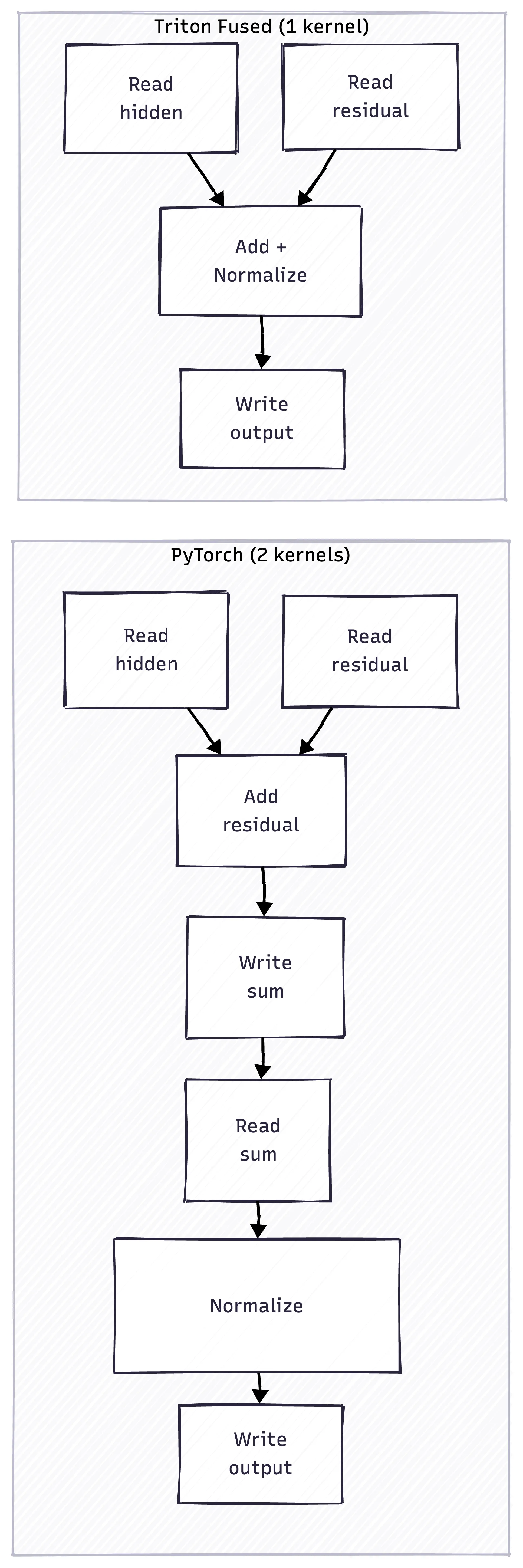
The red boxes show unnecessary memory writes that fusion eliminates. The fused kernel runs 6x faster than PyTorch’s separate operations.
INT8 Quantization: Memory Savings Over Speed
We also implemented INT8 matrix multiplication. The speedup is minimal - maybe 1.04x. But that’s not the point.
The point is memory savings. INT8 weights are half the size of FP16. For a 70B model, that’s the difference between fitting on one GPU or needing two.
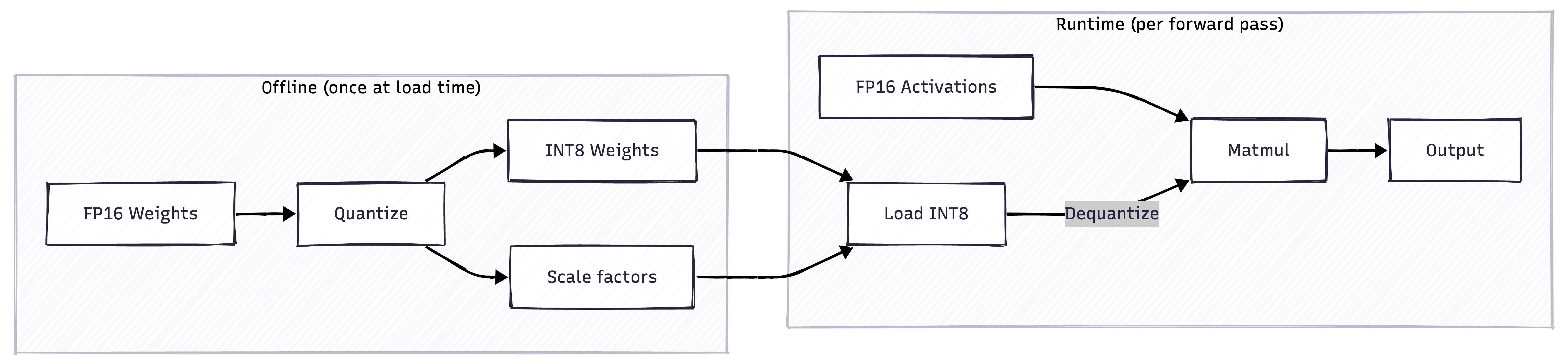
The trade-off: you dequantize on-the-fly during inference. The overhead is why speedups are minimal. But for memory-constrained deployments - edge devices, cost-sensitive cloud instances - INT8 makes models deployable that otherwise wouldn’t be.
Who Benefits From This
This work matters most for teams running inference at scale:
Financial services firms processing thousands of document analysis requests per hour. When each request costs $0.03 in compute, 8x efficiency means the difference between a viable product and a money pit.
Insurance companies running fraud detection or claims processing. High volume, strict latency requirements, and CFOs who scrutinize every cloud dollar.
Healthcare organizations deploying clinical AI. Regulatory requirements often mean on-premise deployment where GPU capacity is fixed. Efficiency determines throughput.
Any enterprise where AI inference has moved from experiment to production line item. Once you’re spending $50K/month on inference, optimization isn’t academic - it’s mandatory.
What This Means for Your Architecture
A few principles emerged from this work:
1. Measure bandwidth, not FLOPS. For memory-bound operations (most of inference), GB/s matters more than TFLOPS. Your GPU utilization dashboard might look healthy while actual bandwidth utilization is 11%.
2. Profile before optimizing. We assumed attention was the bottleneck. It wasn’t - normalization and activation functions were worse on a per-operation basis because they’re called more frequently.
3. Fusion opportunities are everywhere. Any time you see sequential operations in a transformer block, there’s probably a fusion opportunity. Residual + norm. Attention + projection. Gate + activation.
4. Don’t roll your own for production (usually). We built these kernels to understand the problem deeply and to integrate them into Accelerate. For most teams, using optimized inference frameworks like vLLM or TensorRT-LLM is the right call. The exception is when you have specific workloads those frameworks don’t optimize well - which is where Accelerate comes in.
How Accelerate Uses This
These kernels form the foundation of Accelerate, our inference optimization layer. But raw kernel performance is just the start.
Accelerate also handles:
- Automatic kernel selection based on input shapes and GPU architecture
- Speculative decoding integration for autoregressive speedups
- Dynamic batching to maximize throughput under variable load
- Quantization-aware routing that picks the right precision for each layer
The 8x kernel speedup compounds with these other optimizations. In production deployments, we typically see 3-5x end-to-end cost reduction - not just on individual operations, but on the full inference pipeline.
The Bottom Line
PyTorch is leaving 89% of your GPU’s memory bandwidth unused on common operations. Custom Triton kernels can close that gap.
For RMSNorm - an operation that runs hundreds of times per LLM request - we went from 11% to 88% bandwidth utilization. 8x faster.
That’s not a rounding error. At scale, it’s the difference between AI that’s economically viable and AI that gets killed in the next budget review.
Inference costs eating your AI budget? Let’s talk about what Accelerate can do for your workloads.